Bayesian Probability Modeling
Most of this analysis is adapted from Bonham-Carter, 1994, Geographic Information Systems for Geoscientists, Pergamon.
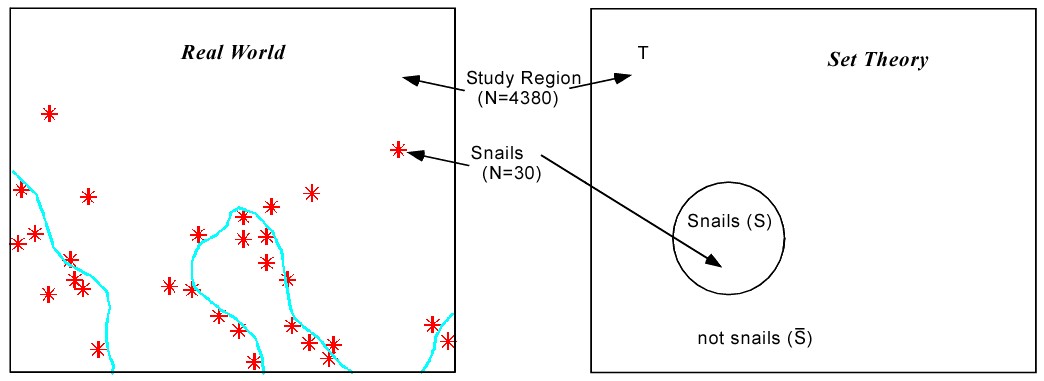
Without any other knowledge, we can assign the probability of finding or being located on “rare snails” (S) cells in the total area of our study (T) as
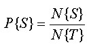
where
- N{S} = number of snail cells
- N{T} = number of cells in the study region
For our “rare snails” example, there are 30 snail cells in 4380 total cells. So the probability P{S} = 30/4380 = 0.0068. This is known as the Prior Hypothesis or the Prior Probability.
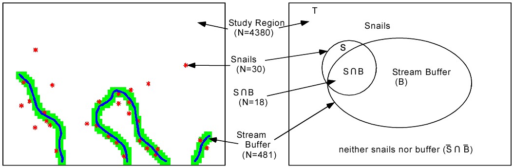
But we know that the snails are by the river, so we can use more information. Thus we can state the probability as “What is the probability of finding snails given that you are in the binary stream buffer (B).” This is written
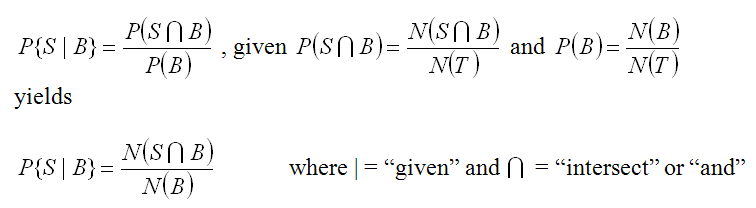
For our example buffer of 45 m, we have P{S|B} = 18/481 = 0.037 and it looks like this in our example. More than half of the snails are in the buffer and the buffer is a much smaller size. So if we are in the buffer our chances of finding a snail go up 5.5 times (.037/.0068).
Now we’d like to do this for more than one “factor” that better explains our snails. We can add aspect. However, using the above method leads to very complicated math. So we change our approach to modify this Posterior Probability in terms of a the Prior Probability times a multiplication factor that represents how much probability increases given the factor. This only works if ALL the factors are INDEPENDENT.
What we need to figger is the “conditional probability” of being in the buffer, given the presence of a snail, and then use that to find out how much advantage being in the buffer conveys to the prior probability. The math is as follows
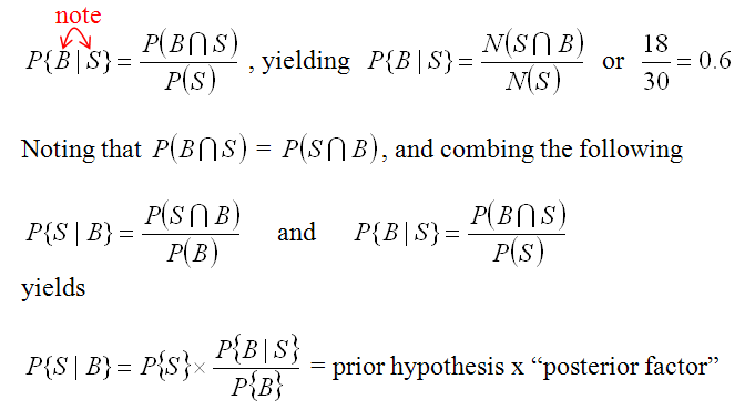
which is for our example = 0.0068 * 0.6 / (481/4380) = 0.037 or = 0.0068 * 5.5 Adding additional variables is easy now that we can simply modify the prior probability with as many posterior factors as is appropriate (again, remembering that each posterior variable must be independent).. Here we can calculate the conditional probability given the presence of the buffer (B) and aspect (A), and etc.
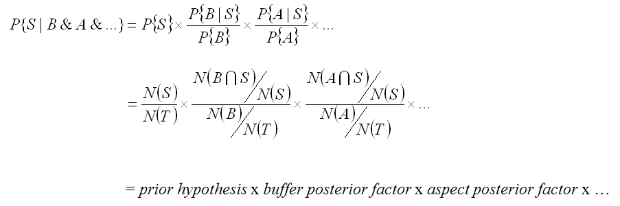
In the excel file in the fuzzy folder, you’ll find data for the calculations of the posterior factor for a 45-m buffer and 4 aspects class. SW had the 2nd highest count of snail cells; should you include SW in your more likely aspects? The data suggest that given a 45 m buffer and a NE aspect, likelihood of finding a snail increases by almost twenty times! (5.5*3.3)
Now we can return to the question of how to choose the buffer for our rare snails example. We can use the “posterior factor” to answer the question: “How do you make a probability buffer (a data-driven fuzzy boundary) where the buffer size represents the probability that you’d include the snails? ” See the last tab in the excel document. Where would you cut off the buffer? Was 45 a good choice? the best choice? You can even take all these probabilities and put them back into your GIS analysis by joining them to the layer (or you might be able to calculate them there??