The goal of unsupervised classification is to automatically segregate pixels of a remote sensing image into groups of similar spectral character. Classification is done using one of several statistical routines generally called “clustering” where classes of pixels are created based on their shared spectral signatures. Clusters are split and /or merged until further clustering doesn’t improve the explanation of the variation in the scene. 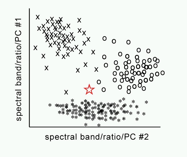
The success of clustering is measured by the “between cluster” versus “within cluster” variability, maximizing the former and minimizing the latter. Given the above illustration, we could easily cluster the pixels into the x, o and * clusters. But how do we get there?
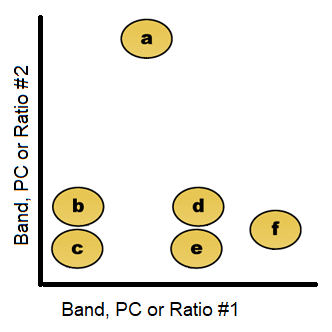
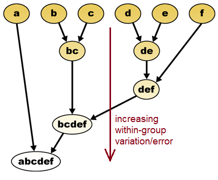
The first diagram (edited from https://en.wikipedia.org/wiki/Hierarchical_clustering) illustrates how the euclidean distance in spectral space (a band, pc, or ratio value) could be used to group pixels, with varying within group and between group variation. This example is visualized with just 2 spectral layers, but the process can use many different layers of information, from raw bands or processed information, or even other grid data like a DEM. The 2nd diagram is similar to a dendrogram. The decision of where to stop splitting or joining groups is usually a “fuzzy” decision based on change in the relative increase of classification precision. (see http://en.wikipedia.org/wiki/Data_clusteringn). If you have had a statistics course, this process is similar to the “Analysis of Variance” techniques wherein one uses the within and between group variability to assess the ability to distinguish between them.
The “classification routines available in ArcGIS Pro are
- ISOCLASS
- Maximum Likelihood
- Random Trees
- Suport Vector Machine
Only 1 is “unsupervised. The rest required training regions and are there “supervised,” which follows in the next topic.
ISO cluster
If we try this ISO cluster unsupervised classification on the strong topography of the VA clip, we wind up with a lousy classification where shadows control the output
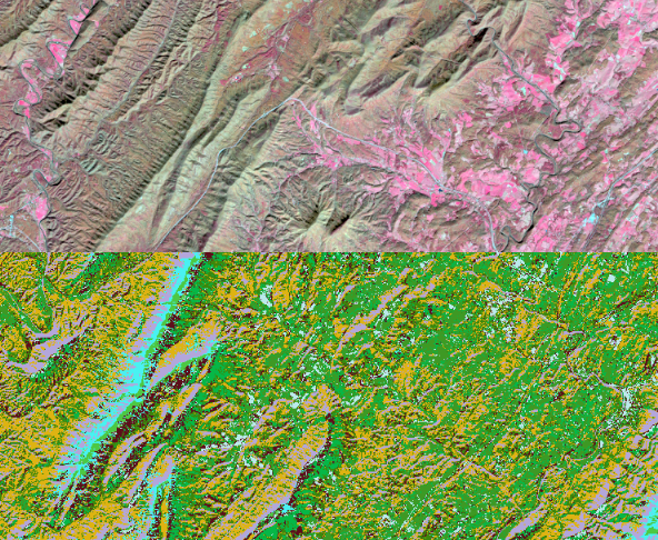
but if we input PCs 2 through 7 into the classifier (or ratios?) things might look better. We’ll try to composite PCs and ratios to see how we do.