Principal-Component Analysis
Because of band correlation, what one sees in Band 1 is not so much different from what one sees in Band 4. If we “decorrelate” all useful bands at once we perform a “principal-components” analysis. For those of you who have had linear algebra, we’re making Eigenvectors where the Eigenvalues contain the contribution of each band to each principal component or Eigenvector.
For this two band mathematical “space,” imagine creating two new axes that describe the maximum variability of the two bands together (b2=m*b1+int). The slope (m) is the measure of the correlation of the two bands (0= no relation, positive = both increase, negative = one increases as the other decrease).
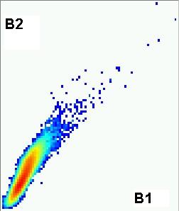
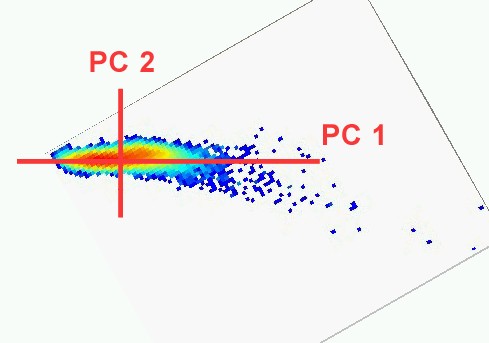
Then we can add a second “component” that is perpendicular to the first.
Now ! Imagine this in 3d, or in 5, 6 or 7 dimensions, which includes all of the bands one wishes to analyze.
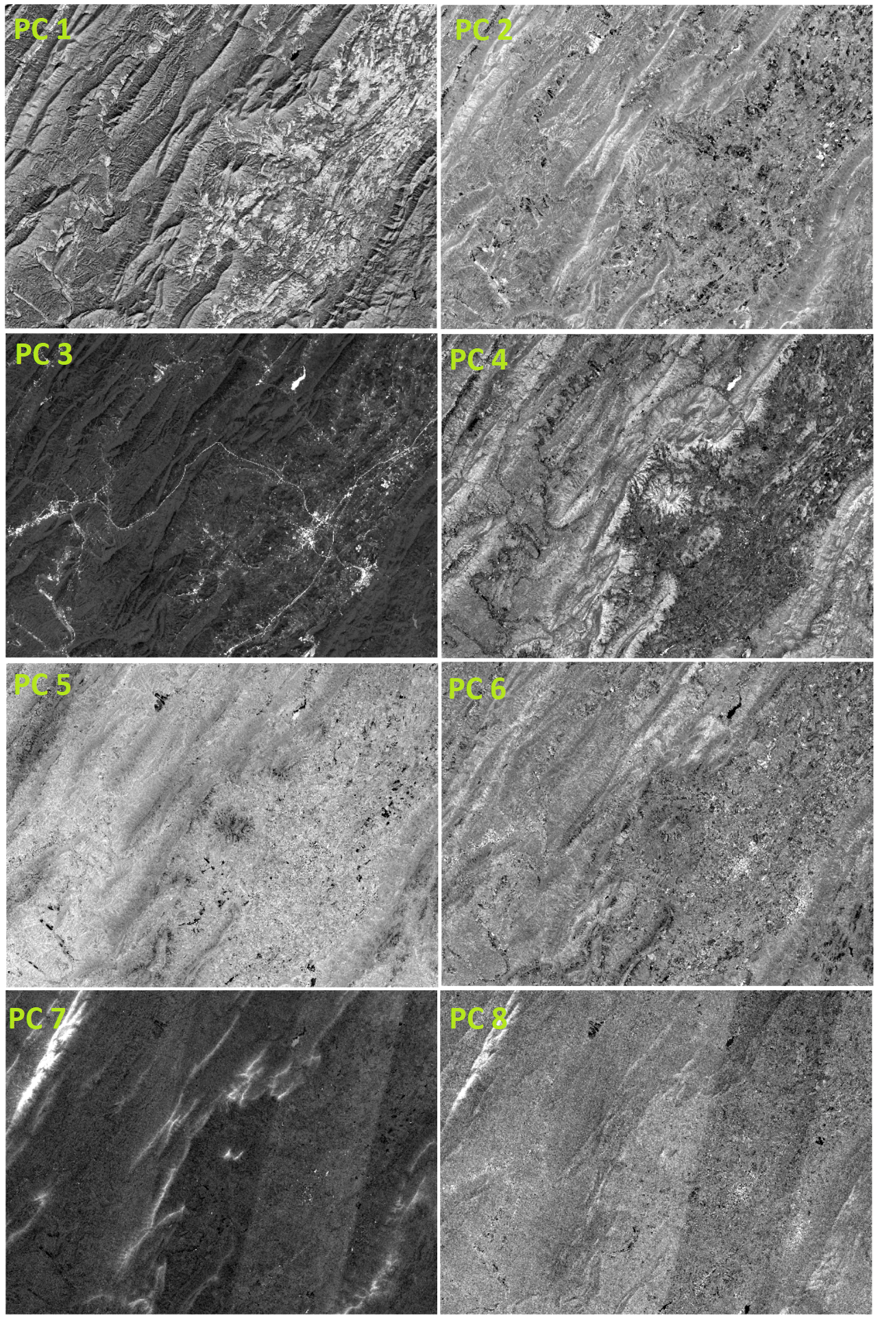
Here are the principal components for the Virginia clip in the satellite_demo project. (from this Landsat image LC08_L1TP_017034_20161105_20170219_01_T1_MTL)
What would be better? Using ratios as inputs for principal components? or raw bands?
In ArcGIS Pro, use the Principal Components tool on the Landsat 8 Virginia clip. You’ll make a text file. I’ve copied some of that output below. Using the output of the principal components (the 8 band dataset), write a list of what is creating strong positive and negative values in each of PC 1 – 6 or 7. What are you seeing (use the swipe tool over your RGB432 image). I have highlight strong (abs(eigenvalue) > 0.2) positive and negative values as red and blue, respectively.
| Eigenvalues | ||||||||
| 7585491 | 1082587 | 108974.1 | 22636.84 | 8765.746 | 2466.671 | 575.283 | 236.5661 | |
| Eigenvectors | ||||||||
| PC | PC 1 | PC 2 | PC 3 | PC 4 | PC 5 | PC 6 | PC 7 | PC 8 |
| OLI Band 1 | 0.040 | 0.036 | 0.373 | -0.115 | 0.465 | 0.391 | –0.208 | 0.658 |
| OLI Band 2 | 0.054 | 0.052 | 0.441 | -0.132 | 0.416 | 0.300 | 0.288 | -0.661 |
| OLI Band 3 | 0.111 | 0.031 | 0.531 | -0.076 | 0.120 | -0.824 | -0.003 | 0.082 |
| OLI Band 4 | 0.130 | 0.198 | 0.445 | 0.752 | -0.377 | 0.188 | -0.042 | 0.003 |
| OLI Band 5 | 0.738 | -0.665 | 0.013 | -0.023 | -0.088 | 0.072 | -0.003 | -0.002 |
| OLI Band 6 | 0.575 | 0.560 | -0.388 | 0.206 | 0.386 | -0.114 | 0.017 | -0.009 |
| OLI Band 7 | 0.301 | 0.447 | 0.191 | -0.595 | -0.540 | 0.158 | -0.040 | 0.020 |
| OLI Band 9 | 0.003 | 0.008 | -0.016 | 0.019 | -0.072 | 0.010 | 0.933 | 0.352 |
How much does each contribute? And what do they identify?
| PC | EigenValue | Percent of EigenValue | Cumulative Sum | What is being imaged in this PC? |
| 1 | 7585491 | 86.084 | 86.084 | |
| 2 | 1082587 | 12.2857 | 98.3697 | |
| 3 | 108974.1 | 1.2367 | 99.6064 | |
| 4 | 22636.84 | 0.2569 | 99.8633 | |
| 5 | 8765.746 | 0.0995 | 99.9628 | |
| 6 | 2466.671 | 0.028 | 99.9908 | |
| 7 | 575.283 | 0.0065 | 99.9973 | |
| 8 | 236.5661 | 0.0027 | 100 |