In this exercise, you’ll learn about creating new data that you’ll use in your next project. We’re going to digitize the relevant parts of the BV and Glasgow Geologic maps (by Dr. Edgar Spencer, former Geology professor and dept head). To do that you have to learn to “georeference” scans of maps and use the polygon and “autocomplete polygon” tool to construct the geologic polygon feature class from it.
The steps are
- georeference or “warp” a scanned image of the geologic map to the same projection as the topographic map data (using the georeferencing tools in ArcGIS). Instructions are on this page and lab (“snips”) report instructions are in the word doc.
- digitize the geology polygons
- first, complete a portion of Bolstad Lab 3 that deals with polygon digitizing (in Bolstadlab3 folder see pdf for instructions)
- then, digitize a portion of the geologic map as a new feature class
- merge the tiles (after each tile is assembled) – Instructions below.
- dissolve the geology units across the separate tiles – Instructions below.
- assess the precision and accuracy of this work.
To start: Copy the box folder 2024GIS_sharedwork\exercises\exercise5\digitize to your box folder or P drive folder, then start a new ArcGIS project in that folder.
Warning: The map frame, data layer from which you are digitizing (geo map), and any new data layers must ALL be in the same projection.
The Geology Map
Below is what you’ll input into the team geology map (all are depending on you, you’ll have to pull your weight on this). The map in the background is the seamed together topographic quadrangles for this exercise (“bv&glasgow24kdrgs.jpg”) that will serve as the base for your new data.
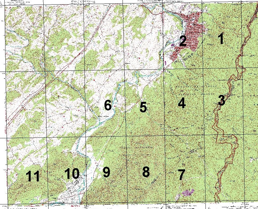
The scans for each numbered section are in the folder geo_maps. Copy just your assigned map to your digitize folder. The pdf of the original geology maps is also in the folder so you can better see the units. Use the pdf to see anything that doesn’t show up well in the scan (like the unit that goes with the color you’re digitizing).
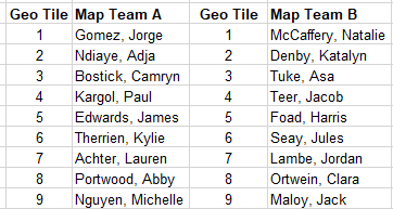
Student & Team & Map Tile number (Dave will do tile 10 and we’ll skip 11)
Georeferencing the jpg image (aligning the scan of the geology map to a projected or “geolocated” drg (“digital raster graphic” or “image”) of the BV and Glasgow topo maps
- Look through these general descriptions of the ArcGIS georeferencing (including “warping“), but the specific steps are on this page. Lots of links to follow in the help menu (at left in the above pages) for additional help!
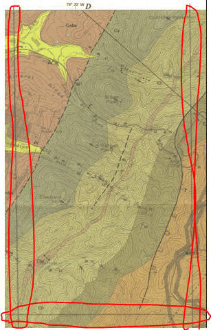
- Examine the projection and cell size information for the DRG called “bv&glasgow24kdrgs.jpg” in the digitize folder
— Note that the digital file is not the projection of the paper maps, which are polyconic, NAD1927 datum, but how the digital scans of these paper maps are projected in digital form.
Note: This is two USGS 7.5 map images collared and stitched together using called a program called ERMapper, which we don’t have anymore. - Insert a new map frame and load the quadrangle jpg image. Check the coordinate system of the map and image, again. Make sure they’re the same.
- Import the map tiles shapefile to your database and then add it to the map.
- Under the “list by selection” tab in the table of contents panel (at the top), uncheck the “map_tiles” layer.
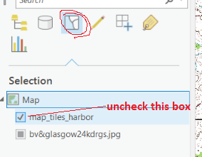
Now move to the editing (pencil) tab and uncheck it there too.
These actions keep you from accidentally selecting, editing or moving items on this layer. We need it to stay unedited, because we will each “snap” to during the digitizing of the geology maps. - Right click on the “map_tiles” layer and check “label features” and tile numbers will be displayed. Zoom in to an area that is centered on and a little bigger than the tile assigned to you. Adjust the shape of the ArcGIS pro window so that your map window won’t be your entire landscape screen……
- Add the .jpg scan of your part of the geologic map from your folder.
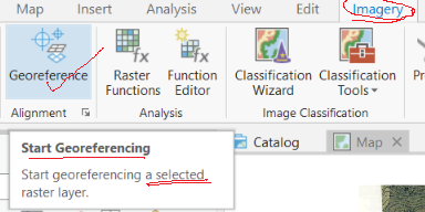
It will warn you that it can’t be projected, but we know that, because it is just a scan without coordinates so far. - Select the geol map scan in the table of contents and from the imagery tab. (And make sure it stays selected, because that’s the layer being edited–don’t edit the coordinates of the reference layer (the topo map)!). Then select the georeference tool on the the imagery tab (note what it says in the help files about saving!).
- Perform steps 6 and 8-10 in the help website.
- Make “control point” pairs (one set of coordinates will be in pixels on the image, and the second set of the pair will be the UTM coordinates where you want it to be) by “add control points” button then click first on the image point of comparison (the green cross), then second on the topo map point (red cross) of comparison (shown below as the same intersection, with geo map transparent over the topo map). You can zoom and turn layers on or off between the two clicks, if that helps. Make sure you can see same feature on both the reference topo image and the geo map image you are georeferencing before you start.
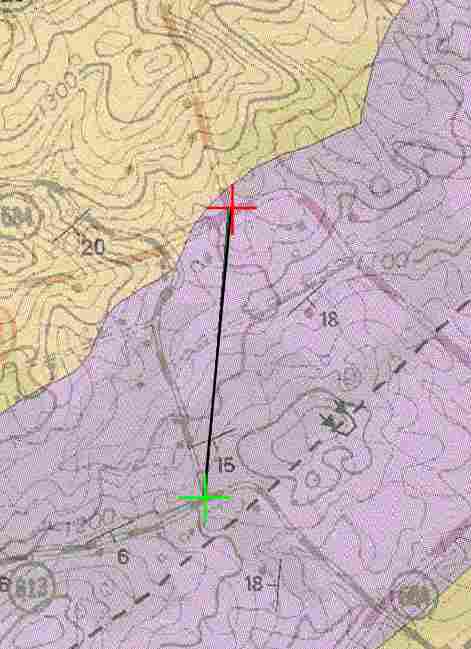
Move around to get points near the map corners and then fix the middle if necessary. Do not use the straight pencil lines on the scan for control points; they do not exactly match the lines in the map_tiles layer. If you make a mistake, finish the collection of that data pair, open the table from the Georeferencing toolbar (“Control Point Table”) and delete the last point. DO NOT USE CTRL Z because this might do something like remove your scan and all the data with it. As you collect points, open the table and save the file of points to your homework folder or geodatabase (I forget which). Do this often and especially when you are finished with the rectification. This is also a good piece of metadata, and you should note the RMSE for your metadata . RMSE is given in the units of the destination for the transformation. Do you know what the cell size is of the topo map? Your error should approach the cell size of that raster, but it won’t likely be less than the cell size.
–Post a couple of snips of your control points with the geology transparent over the topo map.
–And when you’ve got all you need, post one zoomed out showing them all.
–Post a snip of your final Control Point Table with the RMSE - Georeferencing or Geolocating. When you’re satisfied, set the transformation to something that works well (you shouldn’t have to “warp” it much. It is a UTM-like map already). Save the location data to your jpg image with “Save”, then “Save As New” with a good name to your folder or to your geodatabase. If it asks, in the export tool, choose the “Nearest Neighbor” but I would definitely use the lowest order of transformation (likely 1st order affine: rotate and scale only, or “adjust”).
See the notes page here on “Geolocating images” if you have questions.
Digitizing the Geology
- First complete the polygon portion of Bolstad’s lab three. Then return here to digitize the geology for your tile
- As you digitize the outlines of the geologic units, input use these unit values for each polygon you’re creating. When all of the tiles are done and put together, you can join the csv table by unit to get Geology and Lithology on your attribute table.
Unit Geology Lithology 1 Qal* Alluvium 2 td Terrace Alluvium 3 Ost Carbonate 4 Cco Carbonate 5 Ce Carbonate 6 Cwbs Shale 7 Ca Sandstone 8 Ch,Chs Sandstone 9 Cu Phyllite 10 Yb, Yl, Cz crystalline *include the river (digitize right through it) - Did you remember to turn off the “selection” and “edit” tabs for the “map_tiles” layer? Don’t edit that layer by accident; many have in the past to ill effect.
- Create a new polygon feature class in your project geodatabase with the following info.
- Name your new map AorB_geo##_username where Aor B is your team, ## is your map tile number above (01, 02, etc, please use the leading zero for 1 to 9) and “username” is your last name.
- Note: Make sure to set the coordinate system! It should be exactly the same as the map view and data in the open project. If you digitize from a projected data layer (e.g., a NAD-83 data layer projected into a NAD-27 data frame) you rely on the “on-the-fly” reprojection routines that may induce errors of several hundred meters at some locations on the map, even though the location distance between the two datums is just 20-30 meters.
- Set up the following field in your new Feature Class to hold the geology unit
- Unit (short integer)
you can join the names and descriptions later using the Geo_Units_Table.csv file in the digitize folder.
- Unit (short integer)
- Select the new feature class and go to the Editing tab.
- Set the snapping environment as directed here (http://pro.arcgis.com/en/pro-app/help/editing/enable-snapping.htm) making sure that the point, end, vertex and edge “agents” are on. You can mess with other options (distance, color, etc) as you like.
- In the table of contents, “List by Snapping” pane, make sure that the map tiles layer in addition to your geology polygon is enabled for snapping (but turned off for selecting and editing!).
- Digitizing
- Start in one corner of your map with a regular polygon, and then work outward by appending new polygons to the previous ones (Auto Complete Polygon) like you did in the Bolstad lab. See Complete Adjoining Polygons in help.
— Post a snip of your first polygon - Do not digitize complete polygons next to each other! They need to “share” the line between them.
–Post a snip of one of your first few appended polygons. - Please make sure your digitizing snaps to the map_tile layer, so that when we merge the data, no “slivers” will be formed.
Note that the “map_tile” lines do not exactly match the pencil lines on your scan of the geology map–those were simply a guide for my scanning.
The map_tile lines are where you should start and stop your map digitizing for your tile, not those circled above on one of the scans of the geo map. - Save edits often! (saving the project doesn’t save the edits to the feature class to the geodatabase–the save in the edit toolbar does)
- Post a snip of your digitized geology tile overlain on your georeferenced scanned geology map.
- Make sure all your edits are saved. Then copy your feature class to the shared geodatabase geo_maps_2024.gdb.
- Right-click on the “Folders” in the catalog pane
- “Add a folder connection”
- Migrate to the Box folder and select the “2024GIS_completed_geo_maps” (do not open it)
- Click “OK”
- You should now be able to open your geodatabase in the Catalog Pane, right click on your feature class and choose “copy”
- Right-click on the “geo_maps_2024.gdb” geodatabase in that newly added folder and choose Paste.
- once you’ve copied it to the shared geodatabase, Post a snip from the catalog pane showing your tile in the shared geodatabase.
- Please do not delete or remove anything from that folder or geodatabase, if you need to recopy it, please just add a new version of it with a “_v2” at the end.
- Start in one corner of your map with a regular polygon, and then work outward by appending new polygons to the previous ones (Auto Complete Polygon) like you did in the Bolstad lab. See Complete Adjoining Polygons in help.
- Once all of the digitized areas are available, each student will make a single Geology map that covers the entire area, selecting team A or team B (or if one team or tile is a complete mess, only one feature class from each tile 1-10).
- Once they are all complete (I will alert everyone),
copy this Geodatabase to your own project folder (or copy the data out of it into yours). Examine the other students’ efforts and import 10 geology panels into your own project geodatabase (either by team, or if needed, subbing in for a tile from another team).
–Post a snip of the individual map tiles (similar to below) - Merge them using the Merge (data management) Geoprocessing tool (do you know what that tool does? read a bit if you don’t)
–Post a snip of the merged map tiles (similar to below) - Dissolve the boundaries between matching units using the Dissolve (data management not coverage) Geoprocessing Tool. Use “Unit” as the dissolve field.
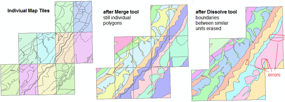
–Post a snip of the dissolved map tiles (similar to above) - Examine it for errors (You can see “fixing topology errors” in the help menu for extra credit) and use these in the “accuracy” discussion.
— Find, zoom in to and post a few snips of errors, including of different kinds, that will need fixing (holes, overlaps, misalignments, incorrect field data, etc) - Post your assessment of the accuracy and precision of this geology layer based on our construction process. Accuracy and precision are two different things; ask if you don’t know.
- Precision should be quantitative, indicating distances in meters.
- How might you assess this for the two processes (georeferencing and digitizing)?
- What kinds of errors are possible (spatial? categorical? topological?)?
- How do you locate errors?
- Five points of this week’s exercise are for how well you georeferenced and digitized your map (precise, mostly error free and in the right place/format)
- Want 10 points extra credit? Fix all the errors in the merged and dissolved map (A or B) using the topology tools and attribute table as necessary. (You’ll likely have to read up about topology tools, see lab template for details)
- Once they are all complete (I will alert everyone),