Creating surfaces from point data by interpolation
With proximity and density, we made grid coverages from discrete data, but the values of the created grids were different than the original data. However, in the example of proximity to rainfall point measurements, we could choose to label the grid with rainfall amount to get a “rainfall surface.” Given point values for any measure (air temperature, nitrate in groundwater, elevation, etc) it is often desirable to create a grid that “fills in” the values between the points. Not a simple thing to do as it turns out.
Things to consider.
- what is the distribution of the points across the surface?
- must the surface fit exactly to the points? (noisy or not)
- how much smoothing is desired? or are you looking for change instead?
- how much complexity of the surface is desired?
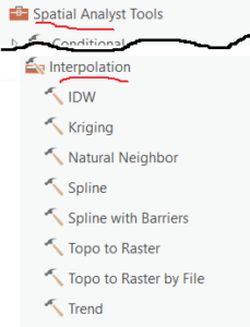
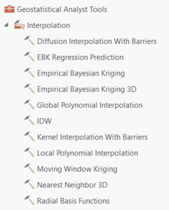
Surface creation (interpolation) tools are in the ArcGIS Pro Spatial Analyst (grid) toolbox and more statistical types of interpolation (e.g., kriging) are also available in a geostatistical toolbox.
Surface types
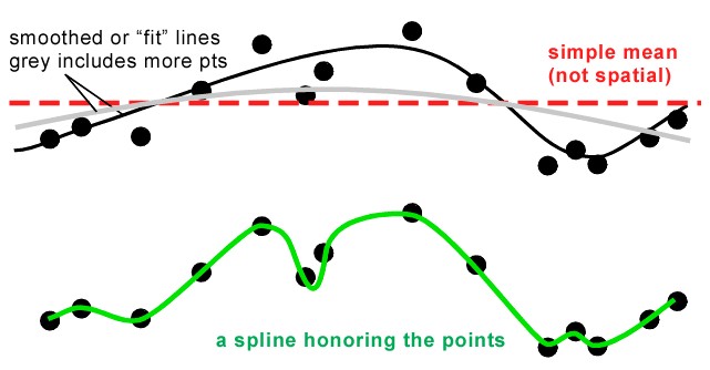
- Simple mean.
This is a non-spatial average of the data in tabular mode. - Smoothed or “low pass” filter.
The high frequency variation (if you think of a radio signal, for example) is removed leaving the low frequency oscillations to “pass” through. To accomplish this you would use the focal statistics tools on a grid, but how about points?- Starting from a grid, we’d use the mean filter (with varying numbers of points or size of the neighborhood) on an existing surface (Neighborhood Statistics...)
- For points, use “inverse distance weighting” , which uses this equation
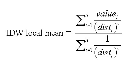
to determine the local value. (see IDW in the ArcGIS help) - Use “Kernel Density” tool but use points that have values to use in the “Population” field. See previous Density topic.
- Use a Spline curve, which is a mathematically-based curvature minimization routine that mimics what people used to do with a thin metal “spline” bent around pins pushed into a plot of data. (see Spline in the Spatial Analyst Functional Reference)
- A Natural Neighbor “stealing” algorithm) starts with a Voroni (Thiessen) polygon and area weights or averages the known values by percent of the unknown polygon.
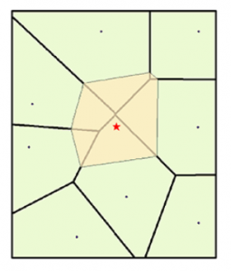
Here the red star is the location of the cell in the grid being interpolated. (from ArcGIS Pro help)
- Edge Enhancement or “high-pass” filters can be applied to points as well as grids. This is accomplished by making a low-pass filter, and then subtracting the low pass filter from the original (called a high pass) and possibly, adding back onto the original values (and edge enhancement). (Can we do this ArcGIS still? Don’t know).

Statistical Methods for Generating Surfaces
The next topic, “Trend” surfaces, should be here, but it is in the Spatial Analyst “Interpolation” toolbox instead.
Here’s a warning (from QGIS) about running tools without knowing anything about statistical analyses of surfaces (and other geoprocessing analyses….make sure you know the subject (statistics, linear algebra, etc) before you start pressing buttons willy nilly.)
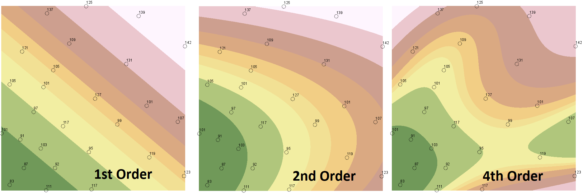
- Fitting polynomial or “Trend” surfaces is just like fitting least squares polynomial regression lines, except that the input are in both x and y. These fitted polynomial surfaces are called “trend surfaces” (see Trend in the Spatial Analyst Help files). This can also be done on categorical layers using a non-parametric “logistic” regression.
- The order of a surface determines the shape. When the shape is linear in x and y (to interpolate z), a flat surface is produced. Higher orders allow curvature.
- The extent and grid cell size are determined by the user to match other surfaces of interest
- Higher order fits can result in extraordinary error at the margins of the predicted surface. Adding points beyond the margin of the area of interest helps control this unwanted behavior.
- Kriging (which I believe is named for a South African ore geologist named Krige) is a process wherein the trend of nearby points is used in the regression. This trend is determined by a variogram, or how the relationship between predictors and predicted values varies with distance and direction on a surface. More information is available at this ArcGIS Pro help page. Spatial autocorrelation and “the range” and “the sill” are of particular interest. See the warning above!
- Geostats wizards have many more techniques to throw at a problem. See the help files or better yet, read a spatial statistics book!